Файл:Karmarkar.svg
Перейти до навігації
Перейти до пошуку

Розмір цього попереднього перегляду PNG для вихідного SVG-файлу: 720 × 540 пікселів. Інші роздільності: 320 × 240 пікселів | 640 × 480 пікселів | 1024 × 768 пікселів | 1280 × 960 пікселів | 2560 × 1920 пікселів.
Повна роздільність (SVG-файл, номінально 720 × 540 пікселів, розмір файлу: 43 КБ)
| Відомості про цей файл містяться на Вікісховищі — централізованому сховищі вільних файлів мультимедіа для використання у проектах Фонду Вікімедіа. |
Опис файлу
| Опис |
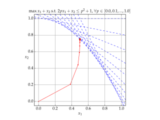
English: Solution of example LP in Karmarkar's algorithm.
Blue lines show the constraints, Red shows each iteration of the algorithm. |
| Час створення | |
| Джерело | Власна робота |
| Автор | Gjacquenot |
Ліцензування
Я, власник авторських прав на цей твір, добровільно публікую його на умовах такої ліцензії:
Цей файл ліцензований на умовах Creative Commons Із зазначенням автора - Розповсюдження на тих самих умовах 4.0 Міжнародна
- Ви можете вільно:
- ділитися – копіювати, поширювати і передавати твір
- модифікувати – переробляти твір
- При дотриманні таких умов:
- зазначення авторства – Ви повинні вказати авторство, надати посилання на ліцензію і вказати, чи якісь зміни було внесено до оригінального твору. Ви можете зробити це в будь-який розсудливий спосіб, але так, щоб він жодним чином не натякав на те, наче ліцензіар підтримує Вас чи Ваш спосіб використання твору.
- поширення на тих же умовах – Якщо ви змінюєте, перетворюєте або створюєте іншу похідну роботу на основі цього твору, ви можете поширювати отриманий у результаті твір тільки на умовах такої ж або сумісної ліцензії.
Source code (Python)
#!/usr/bin/env python
# -*- coding: utf-8 -*-
#
# Python script to illustrate the convergence of Karmarkar's algorithm on
# a linear programming problem.
#
# http://en.wikipedia.org/wiki/Karmarkar%27s_algorithm
#
# Karmarkar's algorithm is an algorithm introduced by Narendra Karmarkar in 1984
# for solving linear programming problems. It was the first reasonably efficient
# algorithm that solves these problems in polynomial time.
#
# Karmarkar's algorithm falls within the class of interior point methods: the
# current guess for the solution does not follow the boundary of the feasible
# set as in the simplex method, but it moves through the interior of the feasible
# region, improving the approximation of the optimal solution by a definite
# fraction with every iteration, and converging to an optimal solution with
# rational data.
#
# Guillaume Jacquenot
# 2015-05-03
# CC-BY-SA

import numpy as np
import matplotlib
from matplotlib.pyplot import figure, show, rc, grid

class ProblemInstance():
    def __init__(self):
        n = 2
        m = 11
        self.A = np.zeros((m,n))
        self.B = np.zeros((m,1))
        self.C = np.array([[1],[1]])
        self.A[:,1] = 1
        for i in range(11):
            p = 0.1*i
            self.A[i,0] = 2.0*p
            self.B[i,0] = p*p + 1.0

class KarmarkarAlgorithm():
    def __init__(self,A,B,C):
        self.maxIterations = 100
        self.A = np.copy(A)
        self.B = np.copy(B)
        self.C = np.copy(C)
        self.n = len(C)
        self.m = len(B)
        self.AT = A.transpose()
        self.XT = None

    def isConvergeCriteronSatisfied(self, epsilon = 1e-8):
        if np.size(self.XT,1)<2:
            return False
        if np.linalg.norm(self.XT[:,-1]-self.XT[:,-2],2) < epsilon:
            return True

    def solve(self, X0=None):
        # No check is made for unbounded problem
        if X0 is None:
            X0 = np.zeros((self.n,1))
        k = 0
        X = np.copy(X0)
        self.XT = np.copy(X0)
        gamma = 0.5
        for _ in range(self.maxIterations):
            if self.isConvergeCriteronSatisfied():
                break
            V = self.B-np.dot(self.A,X)
            VM2 = np.linalg.matrix_power(np.diagflat(V),-2)
            hx = np.dot(np.linalg.matrix_power(np.dot(np.dot(self.AT,VM2),self.A),-1),self.C)
            hv = -np.dot(self.A,hx)
            coeff = np.infty
            for p in range(self.m):
                if hv[p,0]<0:
                    coeff = np.min((coeff,-V[p,0]/hv[p,0]))
            alpha = gamma * coeff
            X += alpha*hx
            self.XT = np.concatenate((self.XT,X),axis=1)

    def makePlot(self,outputFilename = r'Karmarkar.svg', xs=-0.05, xe=+1.05):
        rc('grid', linewidth = 1, linestyle = '-', color = '#a0a0a0')
        rc('xtick', labelsize = 15)
        rc('ytick', labelsize = 15)
        rc('font',**{'family':'serif','serif':['Palatino'],'size':15})
        rc('text', usetex=True)

        fig = figure()
        ax = fig.add_axes([0.12, 0.12, 0.76, 0.76])
        grid(True)
        ylimMin = -0.05
        ylimMax = +1.05
        xsOri = xs
        xeOri = xe
        for i in range(np.size(self.A,0)):
            xs = xsOri
            xe = xeOri
            a = -self.A[i,0]/self.A[i,1]
            b = +self.B[i,0]/self.A[i,1]
            ys = a*xs+b
            ye = a*xe+b
            if ys>ylimMax:
                ys = ylimMax
                xs = (ylimMax-b)/a
            if ye<ylimMin:
                ye = ylimMin
                xe = (ylimMin-b)/a
            ax.plot([xs,xe], [ys,ye], \
                    lw = 1, ls = '--', color = 'b')
        ax.set_xlim((xs,xe))
        ax.plot(self.XT[0,:], self.XT[1,:], \
                lw = 1, ls = '-', color = 'r', marker = '.')
        ax.plot(self.XT[0,-1], self.XT[1,-1], \
                lw = 1, ls = '-', color = 'r', marker = 'o')
        ax.set_xlim((ylimMin,ylimMax))
        ax.set_ylim((ylimMin,ylimMax))
        ax.set_aspect('equal')
        ax.set_xlabel('$x_1$',rotation = 0)
        ax.set_ylabel('$x_2$',rotation = 0)
        ax.set_title(r'$\max x_1+x_2\textrm{ s.t. }2px_1+x_2\le p^2+1\textrm{, }\forall p \in [0.0,0.1,...,1.0]$',
                     fontsize=15)
        fig.savefig(outputFilename)
        fig.show()

if __name__ == "__main__":
    p = ProblemInstance()
    k = KarmarkarAlgorithm(p.A,p.B,p.C)
    k.solve(X0 = np.zeros((2,1)))
    k.makePlot(outputFilename = r'Karmarkar.svg', xs=-0.05, xe=+1.05)
Історія файлу
Клацніть на дату/час, щоб переглянути, як тоді виглядав файл.
| Дата/час | Мініатюра | Розмір об'єкта | Користувач | Коментар | |
|---|---|---|---|---|---|
| поточний | 15:34, 22 листопада 2017 | | 720 × 540 (43 КБ) | DutchCanadian | The right hand side for the constraints appears to be p<sup>2</sup>+1, rather than p<sup>2</sup>, going by both the plot and the code (note the line <tt>self.B[i,0] = p*p + 1.0</tt>). Updated the header line. |
| 19:29, 3 травня 2015 |  | 720 × 540 (41 КБ) | Gjacquenot | Updated constraint display | |
| 19:26, 3 травня 2015 |  | 720 × 540 (41 КБ) | Gjacquenot | Updated constraint display | |
| 19:17, 3 травня 2015 |  | 720 × 540 (41 КБ) | Gjacquenot | Updated constraint display | |
| 18:54, 3 травня 2015 |  | 720 × 540 (41 КБ) | Gjacquenot | User created page with UploadWizard |
Використання файлу
Така сторінка використовує цей файл:
Глобальне використання файлу
Цей файл використовують такі інші вікі:
- Використання в ar.wikipedia.org
- Використання в en.wikipedia.org
- Використання в fr.wikipedia.org
- Використання в ja.wikipedia.org
- Використання в ko.wikipedia.org
- Використання в pt.wikipedia.org
- Використання в ru.wikipedia.org
- Використання в simple.wikipedia.org
- Використання в zh.wikipedia.org